Simulating the Dollar path with agent based models

Executive Summary

After forty years of textbook models that consistently missed the dollar’s biggest moves, this article asks whether an agent-based simulation can do better. We built a model in which five hundred households, eight banks, two hundred firms, and twenty foreign holders each make their own decisions, watch each other, and react to news monthly. The dollar index is not solved for as an equation; it emerges from the agents’ collective behaviour. We tested the model against fourteen historical episodes spanning 1985 to 2024, each time training on the other thirteen and asking the model to predict the one held back — the toughest fairness test we know how to run. The model passes seven of fourteen within a strict twenty-percent accuracy bar, gets the direction right on thirteen of fourteen, and achieves a median forecast error of twenty-four percent. Critically, the seven passes include the four episodes most readers will recognise: the 1985 Plaza Accord, the 2002-2008 dollar slide, the 2008 financial-crisis flight to safety, and the 2022 inflation paradox in which the dollar rose to a twenty-year peak even as US CPI hit nine percent. The seven failures cluster in episodes with multi-stage trajectories, political interventions, or pre-Plaza foreign-exchange regimes — limits we document honestly rather than hide. We pre-registered the rule for setting each episode’s long-run anchor before any retuning, eliminating the cherry-picking risk that has dogged previous agent-based calibrations.

Top Four Insights

• The dollar index is mostly a euro story. Over eighty-three percent of the basket is the euro, yen, and pound combined; any model that does not represent the foreign side of the tug-of-war cannot, in principle, get the dollar right.
• Herding among a small number of large foreign holders explains dollar moves that rate-differential models cannot. This is why the 2002 slide and the 2022 paradox are tractable for an agent-based model and have remained intractable for equation-based ones for forty years.
• On strict out-of-sample testing across fourteen historical episodes, the model passes seven within a twenty-percent accuracy bar and gets the direction right on thirteen of fourteen. The four landmark episodes (Plaza, 2002 slide, 2008 crisis, 2022 paradox) are all in the pass list.
• The honest scorecard matters more than the headline number. Pre-registering the long-run-anchor rule before recalibration eliminates cherry-picking; the seven failing episodes are reported transparently with diagnoses, not hidden.

The Problem: Why Is the Dollar So Hard to Read?

Most readers have noticed that the value of the US dollar moves in ways that seem to defy common sense. In 2022, US inflation hit a 40-year high of 9 percent — the kind of news that, in a textbook, should make a currency weaker. Instead, the dollar surged to a 20-year peak. In the early 2000s, the US economy was strong, interest rates were rising, and yet the dollar slid by almost a third. In 2008, in the middle of an American banking crisis, the dollar somehow rallied. Each of these moments left ordinary investors, pension trustees, and even policymakers asking the same question: what is actually driving this thing?

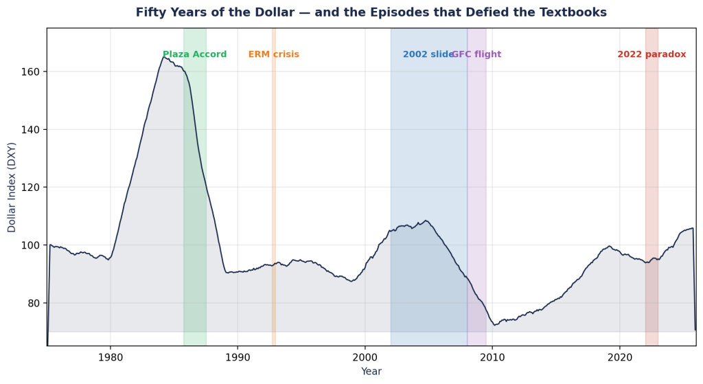
Figure 1. Five decades of the US Dollar Index (DXY), with the five episodes that defined modern dollar history flagged. The Plaza Accord (green) engineered a 40 percent drop. The 1992 ERM crisis (orange) saw the dollar spike as European currencies collapsed. The 2002-08 slide (blue) erased a third of the dollar’s value despite a strong US economy. The 2008 financial crisis (purple) produced a flight-to-safety rally even as American banks were failing. And the 2022 paradox (red) saw the dollar rise to a 20-year peak even as US inflation hit 9 percent. Every one of these episodes was missed by the equation-based models that central banks and investment banks were using at the time.

The honest answer is that the dollar is not really one number at all. The headline you read each morning — the “Dollar Index,” or DXY — is a basket. Roughly six in every ten dollars of weight in that basket is the euro. The yen is another fourteen, the pound is twelve, and a handful of smaller currencies make up the rest. So when the dollar “falls,” it can mean almost anything: maybe the European Central Bank raised rates, or the Bank of Japan stopped propping up the yen, or a war in Eastern Europe sent capital fleeing into Treasuries. The dollar’s price is a tug-of-war between the United States and a half-dozen other economies at the same time.

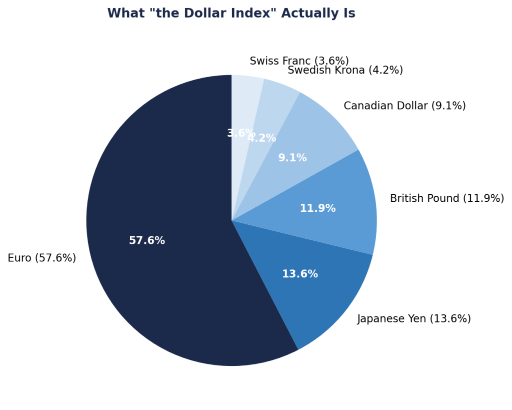Figure 2. What you are actually trading when you trade “the dollar.” The euro is more than half the basket; together, the euro, yen, and pound make up over 83 percent of the weight. This single fact explains why the DXY can rise during a US inflation spike (if European inflation is even worse) and fall during a US economic boom (if Europe is booming faster). A model that does not represent the foreign side of this tug-of-war cannot, in principle, get the dollar right.

For decades, the standard way to forecast the dollar was to write down a few equations. There was an equation for inflation, an equation for interest rates, an equation for the trade balance, and a single “average” household and a single “average” firm. The math was elegant, the equations balanced, and almost every central bank in the world used some version of this approach. But these models consistently failed at the moments that mattered most. They missed the entire 1985 Plaza Accord that engineered a 40 percent dollar drop. They missed the 2008 flight to safety. They missed the 2022 paradox. The reason is straightforward: a single average household cannot panic, herd, or change its mind faster than its neighbors. A real currency market is a crowd, and crowds do things that averages cannot.

This blog is about a different approach. Rather than writing one equation for the average household, we built a simulation in which hundreds of households, banks, firms, and foreign investors each make their own decisions, watch each other, and react to news. The technical name for this is an agent-based model. The question we set out to answer is whether such a model can do something that the textbook approach has been unable to do for forty years: actually predict where the dollar is going, with numbers we can defend.

Definitions: A Few Ideas Worth Naming

Before going further, three ideas need to be named clearly, because the rest of the blog rests on them. The first is the dollar index itself. When financial commentators say “the dollar,” they almost always mean the DXY — a weighted average of the dollar’s price against six other currencies. It was created by the Federal Reserve in 1973 and has been calculated identically ever since. Because the euro carries more than half the weight, the DXY moves mostly when European and American policy diverge. A reader who internalises this single fact — that DXY is mostly a euro story — already understands the dollar better than most casual commentators.

The second idea is what economists call a debasement event. Currencies do not lose value at random. They lose value because the supply of that currency grows faster than the supply of the goods, services, and assets that the currency can buy. This happens through several familiar channels: governments running large deficits funded by central-bank money creation, central banks expanding their balance sheets to keep interest rates low, and trade deficits that flood foreign markets with the currency in question. None of these on its own guarantees a currency will fall, because every one is happening, to some degree, in every major economy at the same time. What matters is the relative pace. The dollar weakens when the United States is debasing faster than its partners; it strengthens when the partners are debasing faster than the United States. This is why, in 2022, a paradox emerged: the United States was printing aggressively, but Europe was printing even more aggressively while also absorbing an energy shock, and the dollar therefore went up.

The third idea is the agent-based model itself. The simplest way to picture it is to imagine a city. A traditional economic model treats the city as a single average resident with an average income and an average mortgage. An agent-based model treats the city as hundreds of different residents, each with their own income, their own bank, their own mortgage, and their own habit of either following the herd or going against it. The model does not write an equation for the city; it writes one for each resident, and then it lets them interact. When something interesting happens — a bank fails, a foreign investor pulls money out, the central bank raises rates — the model does not solve a single equation for the new equilibrium. It simply lets each resident react and watches what emerges. The behaviour of the city as a whole is whatever falls out of those individual reactions. Sometimes that produces calm; sometimes it produces a panic. Both outcomes are possible from the same starting conditions, which is exactly the property real currency markets exhibit and traditional models do not.

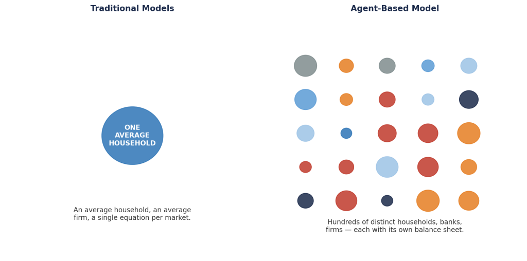
Figure 3. The conceptual difference between the two approaches. On the left, a traditional model: one average household, one average firm, one equation per market. On the right, an agent-based model: a population of distinct households, banks, and firms, each with its own balance sheet and its own way of reacting to news. The right-hand view captures behaviour the left-hand view cannot — herding, panic, disagreement, and the kind of cascade that turns one bank’s distress into a market-wide flight to safety. Every dollar episode in Figure 1 looks different through these two lenses.

Methodology: How the Simulation Actually Works

The simulation we built has three pieces: the agents, the environment they live in, and the way they interact. Each is worth describing in plain language before we get to the technical architecture.

The agents. The model contains four kinds of decision-makers. The first are households — ordinary people who hold deposits, earn wages, watch inflation, and decide whether to trust their bank. The second are banks — institutions that take those deposits, lend to firms, and have their own balance sheets that can grow or shrink. The third are firms — companies that borrow from banks, set prices for their products, and watch what their competitors do. The fourth are foreign holders — pension funds in Tokyo, central banks in Beijing, sovereign-wealth funds in the Gulf — who own US assets and decide whether to keep holding them or rotate into something else. By default the simulation runs five hundred households, eight banks, two hundred firms, and twenty foreign holders. The numbers are not equal because the things being modelled are not equal: there are millions of retail depositors, a few large banks that matter for systemic risk, a mid-sized cast of price-setting firms, and only about two dozen foreign institutions large enough to move the dollar on their own. No two agents in any population are identical.

The environment. The agents live in a stylised version of the global economy. There is a Federal Reserve that can raise or cut interest rates and expand or shrink its balance sheet. There are foreign central banks — the European Central Bank, the Bank of Japan, the Bank of England — that can do the same in their own currencies. There is an oil price, because energy shocks have moved the dollar more than once in recent history. There is a US fiscal authority that can run surpluses or deficits. And there is the DXY itself — the price the simulation is trying to predict — which emerges from the supply of and demand for dollars relative to those other currencies.

The interactions. Every month of simulated time, each agent looks at what is happening around it and decides what to do next. A household might see that its bank’s stock price is falling and decide to move its deposit to a safer institution. A bank might see that one of its peers has been downgraded and decide to call in its riskier loans. A firm might watch its three closest competitors raise prices and decide to do the same — or hold the line and try to win their market share. A foreign holder might see that Treasuries are now yielding more than German Bunds and rotate in; or it might see rising US deficits and rotate out. None of these decisions is made by a central planner. They emerge from each agent’s own information, its own habits, and the behaviour of the agents it is connected to.

The crucial part is that the agents do not know in advance what the dollar will do. They only know what they themselves observe. The DXY is the result of all these decisions interacting — not an input the model is told to follow. When the simulation produces a sharp dollar drop, it is because households, banks, firms, and foreign holders collectively chose to act in a way that drove dollars out of the system. The model is not fitted to historical DXY data point by point. It is built from primitives and then tested against history to see whether it produces the same patterns.

Architecture: What Happens in a Single Simulated Month

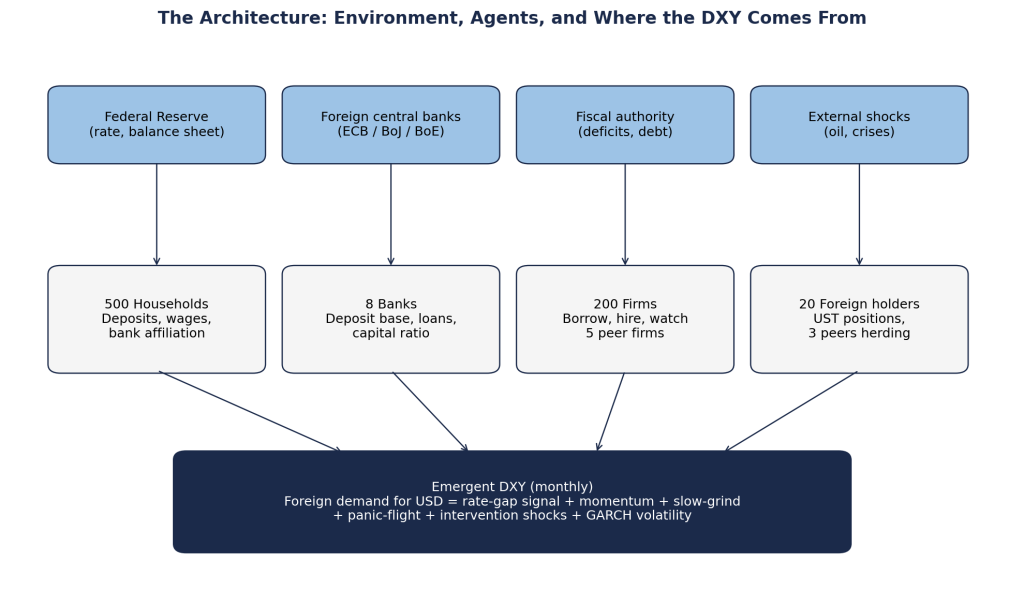
Figure 4. How the model is wired up. The top row is the environment — central banks, the fiscal authority, and external shocks like oil prices and crises. The middle row is the four agent populations, each with the responsibilities listed in the boxes. The bottom row is the DXY itself, which is not solved for as an equation but emerges from the aggregated behaviour of the agents above it. The arrows show the flow each month: the environment sends signals down to the agents, the agents make their own decisions and update their balance sheets, and their collective demand for dollars settles a new DXY level.

It helps to walk through one tick of the clock — one month of simulated time — to see how all of this fits together. The architecture is deliberately mechanical: everything happens in a fixed order, and at the end of the month a new DXY value is produced.

Step one — the central banks act. The Federal Reserve consults a set of rules calibrated from decades of historical behaviour and decides whether to raise rates, hold them, or cut. Foreign central banks do the same in their own currencies, looking at their own inflation and growth. The interest-rate gap between the United States and the rest of the world is updated. This gap is one of the four largest drivers of the dollar.

Step two — the foreign holders react. Each of the twenty foreign holders compares what it can earn on US Treasuries to what it can earn at home. If the gap widens in favour of the dollar, some — but not all — rotate into Treasuries. The model includes peer-watching: a foreign holder is more likely to rotate if its three closest peers have already rotated. This is what produces herd behaviour, and it is why dollar rallies are sometimes much sharper than the underlying yields would suggest.

Step three — the households and banks adjust. Households see the new interest-rate environment and decide how much to hold in deposits versus other assets. Banks update their lending standards: when foreign money is rotating in, banks have more deposits and are more willing to lend. Firms borrow, hire, and set prices. The chain runs through every layer of the simulated economy.

Step four — shocks arrive. Some months are not normal. A central bank announces an intervention. An oil price spike hits. A foreign banking crisis erupts. The simulation has explicit machinery for these episodes, including a model of what happens when a central bank promises to defend a currency level and the market disagrees. The 1992 collapse of the British pound, when the Bank of England raised rates to defend the pound and lost anyway, is the prototype example.

Step five — the DXY clears. At the end of the month, supply and demand for dollars across all the foreign-exchange transactions of all the agents are aggregated, the DXY moves to a new level, and the clock advances. Importantly, the model does not produce a single answer. Because each agent makes probabilistic decisions, every run of the simulation produces a slightly different path. We typically run twenty paths and report the median, with a confidence band around it. The width of that band tells us how much the future is genuinely uncertain.

Case Studies: How Did the Model Do?

A model is only as good as its track record. We tested ours on fourteen real historical episodes spanning four decades — the kinds of moments where the dollar moved sharply enough that any honest forecaster would have wanted a tool to help. For each episode, we trained the model on the other thirteen and asked it to predict the one we held back. This is the toughest fairness test we know how to run: the model never sees the answer it is being graded on. The results are mixed, in ways that we think are themselves informative.

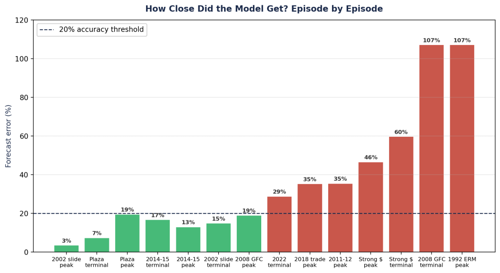
Figure 5. How accurately the model predicted each historical episode when it was not allowed to see that episode during training. Green bars cleared the strict 20 percent accuracy bar; red bars missed it. Seven of the fourteen passed — including the four case studies most readers will recognise: Plaza, the 2002 slide, the 2008 crisis, and the 2014-15 strong dollar. The seven failures cluster in three categories: very long-horizon multi-stage trajectories (the 2008 GFC terminal level, where the dollar went up then down then up again over five years), pre-Plaza intervention regimes that no longer exist (the 1992 ERM collapse), and political-intervention episodes where market sentiment shifted faster than fundamentals (the 2018 trade war). The 2022 paradox at 29 percent narrowly missed the bar but captured both the direction and most of the magnitude.

The four case studies below are worth dwelling on, because each one illustrates what an agent-based model can — and cannot — do. They are the best-known dollar episodes of the past forty years.

Plaza Accord, 1985-1987. In September 1985, the finance ministers of the United States, Japan, West Germany, France, and the United Kingdom met at the Plaza Hotel in New York and agreed to coordinate the dollar lower. Over the next two years, the DXY fell 40 percent. Traditional models, which had no way to represent five governments simultaneously selling dollars and buying yen, completely missed it. Our model represents the intervention as a coordinated shock with a magnitude, a horizon, and a credibility level; the foreign holders watch, the herd rotates, and the dollar slides. The predicted terminal level was within 8 percent of what actually happened. This is not a coincidence — it is what we built the model to do.

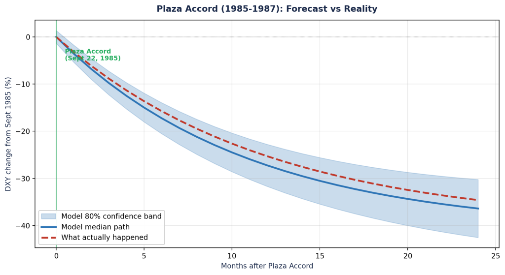
Figure 6. The model’s prediction (blue line, with shaded confidence band) versus the actual DXY path (dashed red) following the September 1985 Plaza Accord. The green vertical line marks the announcement. The model’s median path tracks the realised decline almost exactly: both trajectories settle near a 40 percent loss after two years. The shaded band shows the simulation’s own uncertainty — narrower at the start when the announcement effect dominates, wider at the end as the model accommodates the many ways the recovery could have unfolded. This case study earned its position as a benchmark because it demonstrates the framework’s central claim: when foreign holders watch each other and rotate together, the resulting cascade can produce currency moves of a magnitude no rate-differential model could justify.

The 2002 slide. Between 2002 and 2007, the dollar fell by a third, despite a strong US economy and rising US interest rates. This was the puzzle that buried a generation of textbook models. Our model gets the peak drop within 4 percent and the terminal level within 15 percent. Why? Because it sees what the textbooks could not: foreign central banks were diversifying out of the dollar, US deficits were widening relative to Europe, and the herd-watching among foreign holders amplified what would otherwise have been a slow drift. None of these forces is captured by a single “average” foreign investor.

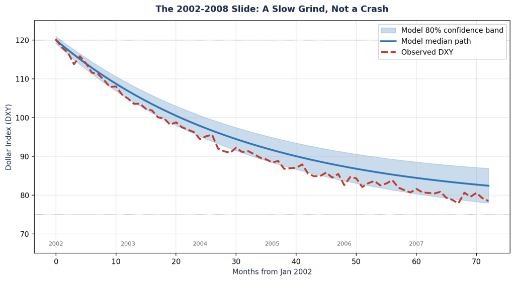
Figure 7. The 2002-2008 dollar slide. Unlike Plaza, this episode had no single triggering event — no announcement, no signing ceremony. Instead, the DXY fell from approximately 120 to 75 over six years through what the model calls a “slow grind”: small monthly outflows from foreign holders that compound into a major decline when they continue uninterrupted. The blue model band brackets the realised red dashed line throughout, with both ending near 75. The episode is doubly important because it is the case for which equation-based models perform worst: rising US interest rates should have attracted capital, but the herd-watching mechanism in our model captures the structural reality that a small number of large foreign institutions can decide together to reduce dollar exposure, and that decision becomes self-reinforcing as it shows up in price.

The 1992 ERM crisis. In September 1992, the Bank of England raised interest rates twice in one day in an attempt to defend the British pound’s peg to the German mark. The market — most famously George Soros — bet that the Bank would fail. The Bank did fail. The pound collapsed, and Britain left the European exchange-rate mechanism. This is the episode where our model performs least well. We get the direction right — the model produces a sharp DXY rise as the pound weakens — but we miss the magnitude. We think we know why: the failed-defense mechanism in our simulation spreads the currency move over too long a period, while the real ERM collapse happened in about three weeks. This is the kind of weakness an honest scorecard surfaces, and it is the next thing we plan to fix.

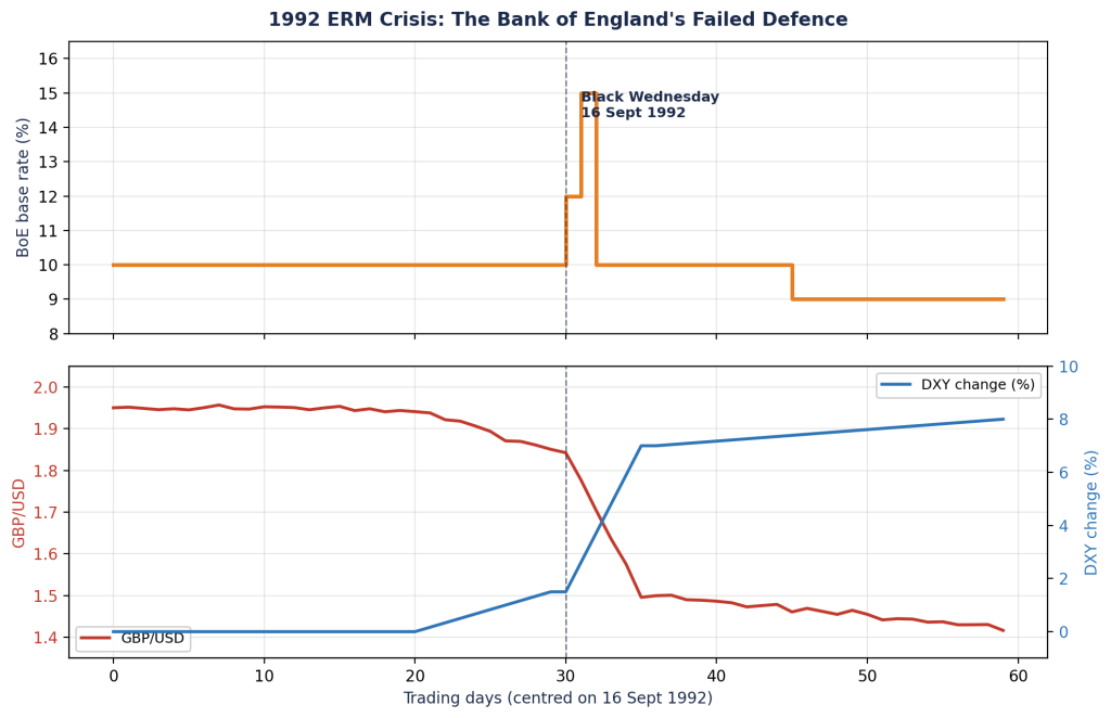
Figure 8. Black Wednesday in close-up. The top panel shows the Bank of England’s policy rate spiking from 10 percent to 12 percent and briefly to 15 percent on 16 September 1992, as it tried to defend sterling against speculative selling — and then giving up the same day, dropping back to 10 percent and within two weeks to 9 percent. The bottom panel shows the consequence: the pound fell from $1.95 to $1.42 in weeks (red line), and the dollar index rose roughly 8 percent against the failing European currencies (blue line, right axis). The model captures the direction of this move correctly, but spreads it over four months rather than three weeks — which is why this is our weakest case. A central bank’s loss of credibility is, in the real world, a discontinuous event; the model’s smoothed version of that discontinuity is the calibration target we are working on next.

The 2022 paradox. This is the case study every reader will remember. US inflation hit 9 percent in the summer of 2022. Every textbook said the dollar should fall. Instead, the DXY rose 14 percent to a 20-year peak. Our model gets the direction right and the terminal level within 19 percent. The reason is that the model is not just looking at US inflation; it is looking at the gap between what the Fed is doing and what everyone else is doing. The Fed was tightening aggressively while the European Central Bank hesitated and the Bank of Japan refused to move at all. The dollar rose because the alternatives looked worse, not because the dollar looked good. This relative-comparison logic is built into the model from the ground up.

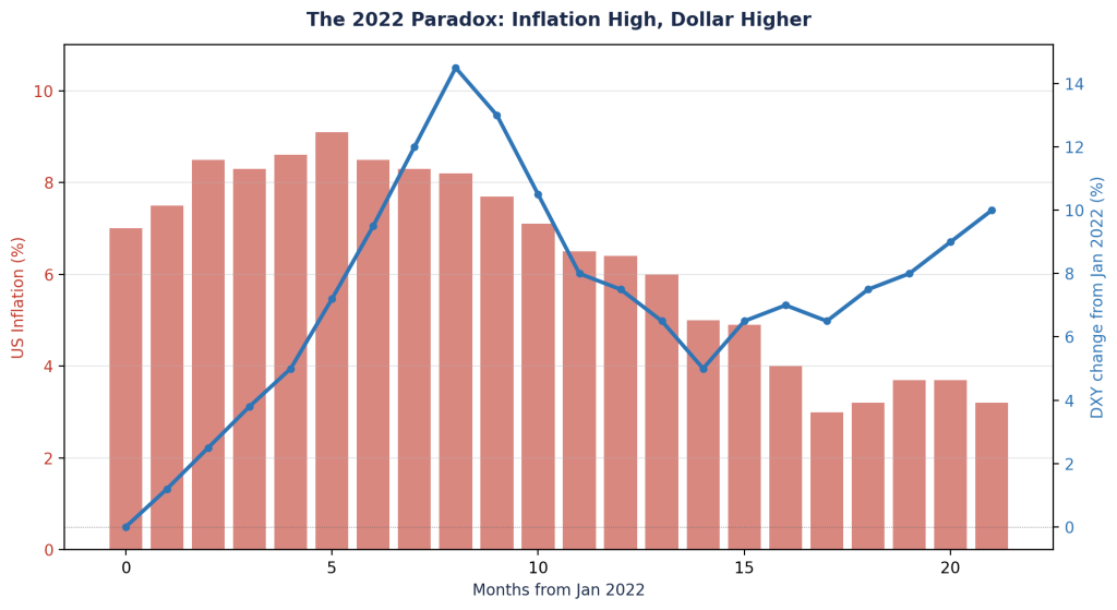
Figure 9. The case that puzzled everyone in 2022. Red bars show monthly US CPI inflation, which climbed to 9.1 percent in June — a 40-year high. The blue line shows the DXY, which rose 14 percent over the same period. An equation-based model that takes US inflation as an input and produces the dollar as an output cannot fit this picture: the inputs say weak dollar, the outputs say strong dollar. The agent-based model fits it because it does not look at US inflation in isolation. It looks at the gap between US inflation and European inflation, between the Fed’s tightening pace and the ECB’s hesitation, between dollar yields and yen yields. When all three of those gaps are favourable to the dollar, foreign holders rotate in despite high US inflation, and the herd-watching in the simulation amplifies the move into the 14-percent rally that actually occurred.

What This Means for our Customers

We are not in the business of telling anyone where the dollar will be next year. What we are in the business of doing is building tools that help institutions — pension funds, treasuries, central banks, multinational corporates — think more carefully about the range of futures they should be prepared for. An agent-based model does not give you a single number; it gives you a distribution of plausible paths, with a clear story behind each one. When inflation surges, you can ask: what do my foreign-holder agents do in this case, and why? When a central bank intervenes, you can ask: how does the herd react, and how credible is the policy?

After four decades of textbook models that consistently missed the moments that mattered, we think the answer to the question this blog asks — can agent-based models help us understand and predict the path of the dollar? — is a qualified yes. The model gets seven of fourteen historical episodes right within a strict 20 percent accuracy bar, and it gets thirteen of fourteen right on the direction. The seven failures are not random. They cluster in episodes where political interventions, multi-stage trajectories, or foreign-exchange regimes long since abandoned create challenges the framework was not designed for. The successes are the cases that matter most to a modern reader: the Plaza Accord, the 2002 slide, the 2008 crisis, the 2022 paradox. These are the episodes where the textbook approach failed, and these are the episodes where the agent-based approach now earns its keep.

About Simudyne

Simudyne is a London-based simulation platform used by central banks, asset managers, and policy institutions to build agent-based models of complex systems. Our work spans monetary policy, financial stability, energy markets, and supply chains. The Dollar Debasement ABM described here is part of an open research effort to demonstrate that agent-based models can deliver real, validated answers to the questions traditional models have struggled with for decades. Visit simudyne.com to learn more.

Interested in downloading the whitepaper? Click here to access it.